paynejoe.com

The discrete Gaussian distribution $D_{\mathcal{L}, r}(x)$ is defined over a lattice $\mathcal{L}$ with parameter $r$ such that the probability of sampling a lattice vector $x \in \mathcal{L}$ is proportional to its weight $$ w(x) = e^{-\pi \|x\|^2 / r^2} $$ where $r$ is the Gaussian parameter, ensures that vectors closer to the origin are more likely to be chosen, which is crucial for many lattice-based cryptographic constructions.

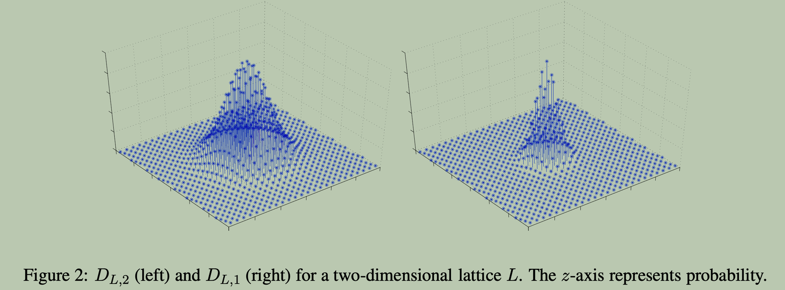
We see that :

• smaller length of vector $x$ is more likely to be sampled.
• smaller parameter $r$ means the distribution is more concentrated around the origin, making shorter vectors more likely to be sampled.

Iteration of Discrete Gaussian Sampling

Given :

1. A lattice $\mathcal{L}(B)$ defined by a basis $B$, and its dual lattice $\mathcal{L}^*(B^{-T})$. They satisfy : $$ \langle x, y \rangle \in \mathbb{Z} \quad \forall x \in \mathcal{L}(B), y \in \mathcal{L}^*(B^{-T}). $$

2. Discrete Gaussian distribution $D_{\mathcal{L}, r}(x)$ with parameter $r$ over the lattice $\mathcal{L}(B)$, which defines the probability of sampling each lattice vector $x \in \mathcal{L}(B)$ proportional to its weight $$ w(x) = e^{-\pi \|x\|^2 / r^2}. $$ By this distribution, we sample a lattice vector $$ v \leftarrow D_{\mathcal{L}, r}(x) $$

3. Target $y \in \mathbb{R}^n$, which is sufficiently close to the dual lattice $\mathcal{L}^*(B^{-T})$.

4. An LWE oracle $\mathcal{O}$.

We aim to find the closest lattice vector $x \in \mathcal{L}^*$ to the target vector $y$, leveraging the discrete Gaussian samples and the LWE oracle $\mathcal{O}$.

Construct LWE Instance

Firstly, We will focus on how to construct a valid LWE instance from the discrete Gaussian samples and the target vector $y$ :

1. Sample a lattice vector $v$ from the discrete Gaussian distribution over the lattice $\mathcal{L}(B)$ with width parameter $r$: $$ v \leftarrow D_{\mathcal{L}, r}(x) $$

2. Recover the modularized scalar vector $a = u \pmod q$ from $v$ : $$ a = B^{-1} v \pmod q $$ , it serves as the LWE instance’s public vector component.

3. Sample a noise $g \in \mathbb{R}$ from the continuous Gaussian distribution with $0$ mean and standard deviation $\frac{\alpha}{2\sqrt{\pi}}$ : $$ g \leftarrow \mathcal{D}(0, \frac{\alpha}{2\sqrt{\pi}}) $$

4. Compute the LWE response $b$ using the target vector $y$, the discrete Gaussian sample $v$, and the noise $g$: $$ b = \langle y, v \rangle / q + g \pmod 1 $$

   Explanation of the response vector

   Since $y = x + h$ where $x$ is the closest lattice vector to $y$ in $\mathcal{L}^*$ and $h$ is the displacement between $x$ and $y$, we have : $$ \begin{aligned} b &= \langle y, v \rangle / q + g \pmod 1 \\ &= \langle x + h, v \rangle / q + g \pmod 1 \\ &= \langle x, v \rangle / q + \langle h, v \rangle / q + g \pmod 1 \end{aligned} $$ Since $x \in \mathcal{L}^*$ and $v \in \mathcal{L}$, where $x = B^{-T} c, s = c \pmod q$ for some $c \in \mathbb{Z}^n$ and $v = B u, a = u \pmod q$ for some $u \in \mathbb{Z}^n$, we have
   $$ \langle x, v \rangle = \langle B^{-T} c, B u \rangle = \langle c, B^{-1} B u \rangle = \langle c, u \rangle \in \mathbb{Z}. $$ We notice that $c$ and $u$ are the scalar vectors of lattice vectors $x$ and $v$ respectively. And since $$ \langle c, u \rangle \pmod q = \langle s, a \rangle \pmod q $$ , thus $$ \langle c, u \rangle / q \pmod 1 = \langle s, a \rangle / q \pmod 1 $$ Therefore, $$ b = \langle s, a \rangle /q + \boxed{\langle h, v \rangle / q + g} \pmod 1 $$ where $e = \langle h, v \rangle / q + g$ represents the effective noise in the LWE response, it should also comes from a fixed Gaussian distribution which is independent of $v$ we sampled.

   
   

The pair $(a, b)$ is an LWE instance with secret $s$ and effective noise $e = \langle h, v \rangle / q + g$, where $a$ is the public vector component and $b$ is the response vector. In order to ensure $(a, b)$ is a valid LWE instance :