
Table of Contents
In complexity theory, we say a problem is hard if it it hard for the worst-case instance; while in cryptography, a problem is deemed hard only if it is hard for the average-case instance (i.e., for all but a negligible fraction of instances).
Basics
Lattice
Definition of a Lattice
Let $\mathbb{R}^m$ be the $m$-dimensional Euclidean (inner product) space. A lattice in $\mathbb{R}^m$ is the set $$ \mathcal{L}(b_1, …, b_n) = \left\{ \sum_{i=1}^{n} z_i b_i \mid z_i \in \mathbb{Z} \right\} $$ of all integer linear combinations of the basis vectors $b_1, …, b_n$, where $n \le m$ is the rank of the lattice, and $m$ is the dimension of the lattice.
Domain of Lattice and Vector Space
Note that the vector (Euclidean) space is defined over field $\mathbb{R}$, but the lattice itself is defined over the integers $\mathbb{Z}$. I think this is a fundamental difference between lattice and general subspace. Because lattice is discrete, it is only restricted to "integer span" of the basis vectors, whereas subspace is defined over the entire field $\mathbb{R}$ and can take arbitrary linear combinations of the basis vectors, which makes it continuous.
Representation of a Lattice
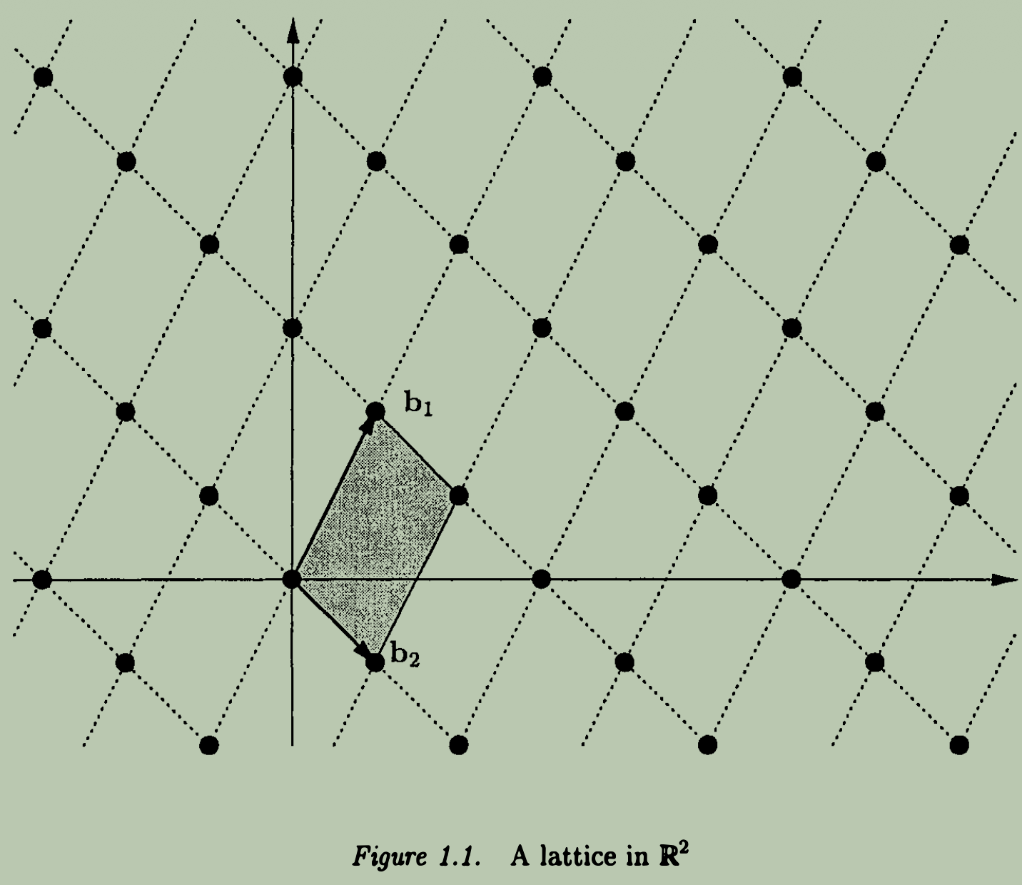
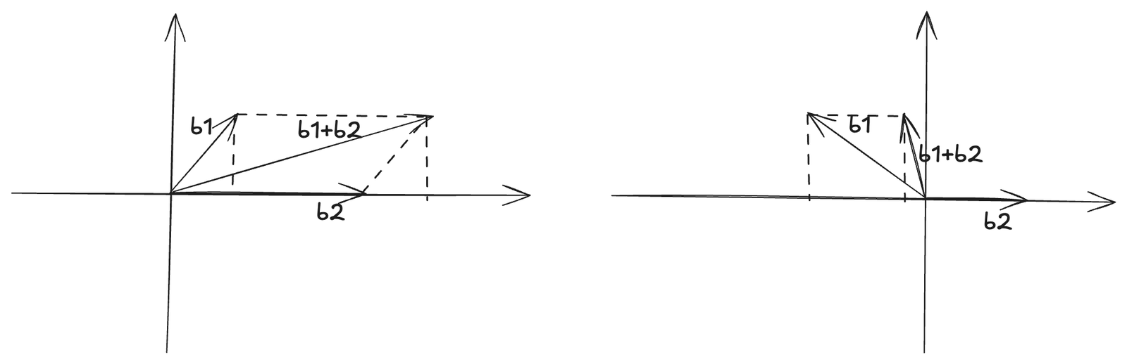
There are many different ways to represent a lattice, depending on the choice of basis vectors. For example, in 2-dimensional space $\mathbb{R}^2$, a lattice can have different bases that generate the same set of points.
| One Basis | Another Basis |
|---|---|
 |
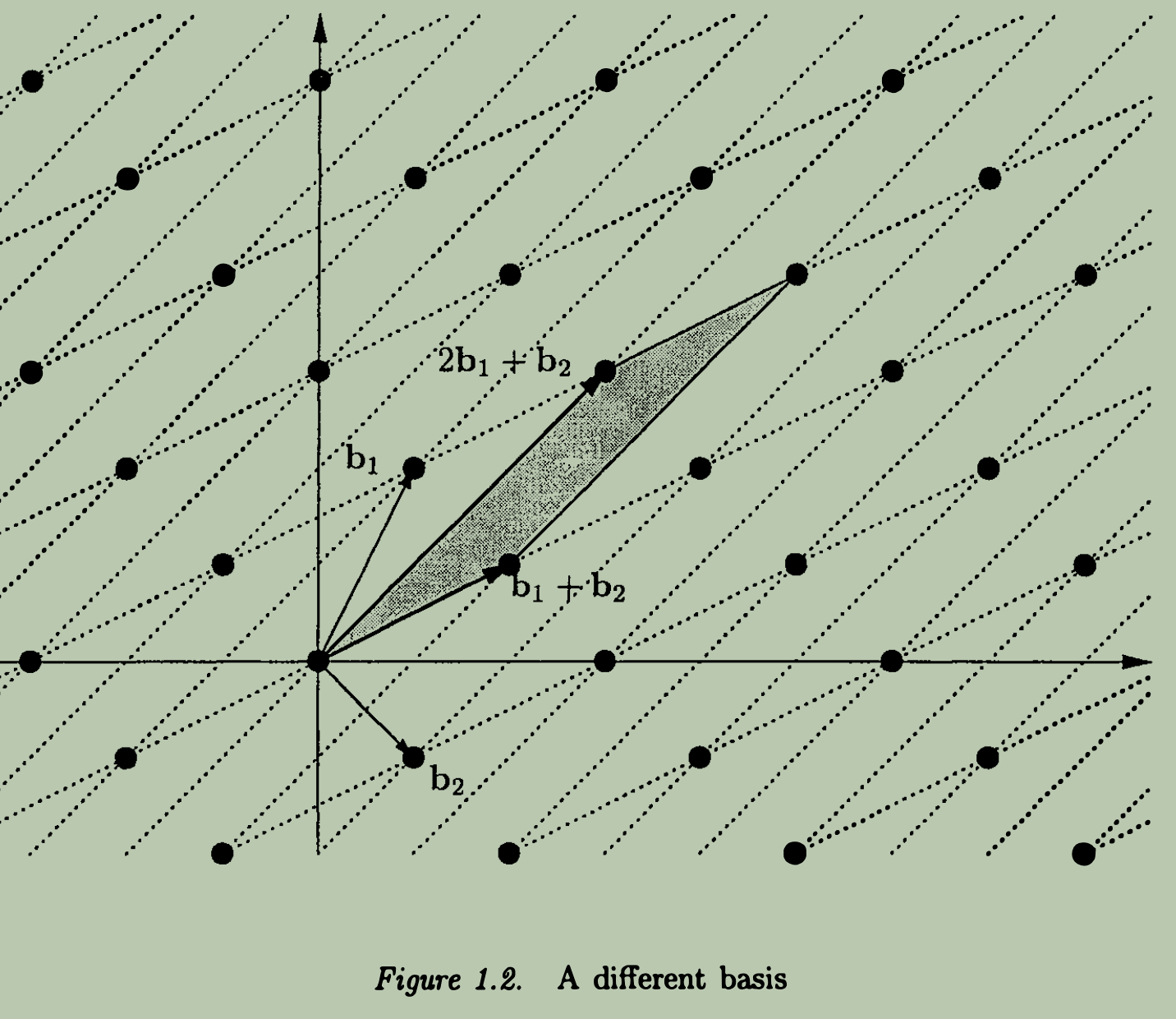 |
Where the left image shows a lattice generated by basis, $$ b_1 = \begin{pmatrix}1 \\ 2\end{pmatrix}, \quad b_2 = \begin{pmatrix}1 \\ -1\end{pmatrix} $$ and the right image shows a lattice generated by another basis, $$ b_1′ = b_1 + b_2 = \begin{pmatrix}2 \\ 1\end{pmatrix}, \quad b_2′ = 2b_1 + b_2 = \begin{pmatrix}3 \\ 3\end{pmatrix} $$ We see that, the (intersection) points of the two lattices coincide, meaning that both bases generate the same set of lattice points in $\mathbb{R}^2$.
Why do different bases generate the same lattice?
One question here : is there any relationships between these bases that generate the same lattice? The answer is yes, if they are related by a unimodular transformation, i.e., an integer matrix with determinant $\pm 1$. That is, $$ >B’ = UB, \quad \text{where } U \in \mathbb{Z}^{n \times n} \text{ and } \det(U) = \pm 1. >$$
We have already noticed that a lattice is defined over the integers $\mathbb{Z}$ which is discrete, whereas the Euclidean space is defined over the field $\mathbb{R}$ which is continuous. Recall that in linear algebra, the $\text{span}(B)$ is independent of the choice of basis $B$, meaning that any basis that generates the same subspace will have the same span. For lattices, different bases can also generate the same lattice.
Fact 1.1 – Span of Lattice Bases
If $B$ and $B’$ generate the same lattice, then $\text{span}(B) = \text{span}(B’)$.
Proof
To show $\text{span}(B) = \text{span}(B’)$, we need to prove two inclusions:
- $\text{span}(B’) \subseteq \text{span}(B)$
- $\text{span}(B) \subseteq \text{span}(B’)$
Regarding (1), since $B’ = B U$ where $U$ is invertible, basis $B’$ is a linear combination of the columns of $B$, meaning that any linear combination of the columns of $B’$ can also be expressed as a linear combination of the columns of $B$. Therefore, $\text{span}(B’) \subseteq \text{span}(B)$.
Regarding (2), since $B = B’ U^{-1}$ where $U$ is invertible, basis $B$ is a linear combination of the columns of $B’$, meaning that any linear combination of the columns of $B$ can also be expressed as a linear combination of the columns of $B’$. Therefore, $\text{span}(B) \subseteq \text{span}(B’)$.
Completing the proof.
Clearly, we see :
-
In this case, lattice $\mathcal{L}(B)$ and vector space $\text{span}(B)$ are closely related, but they are not the same. The lattice consists of discrete points, while the vector space contains all linear combinations of the basis vectors with real coefficients .
-
Any set of $n$ linearly independent vectors from lattice $\mathcal{L}(B)$ forms a basis for vector space $\text{span}(B)$. But this set does not necessarily generate the entire lattice $\mathcal{L}(B)$.
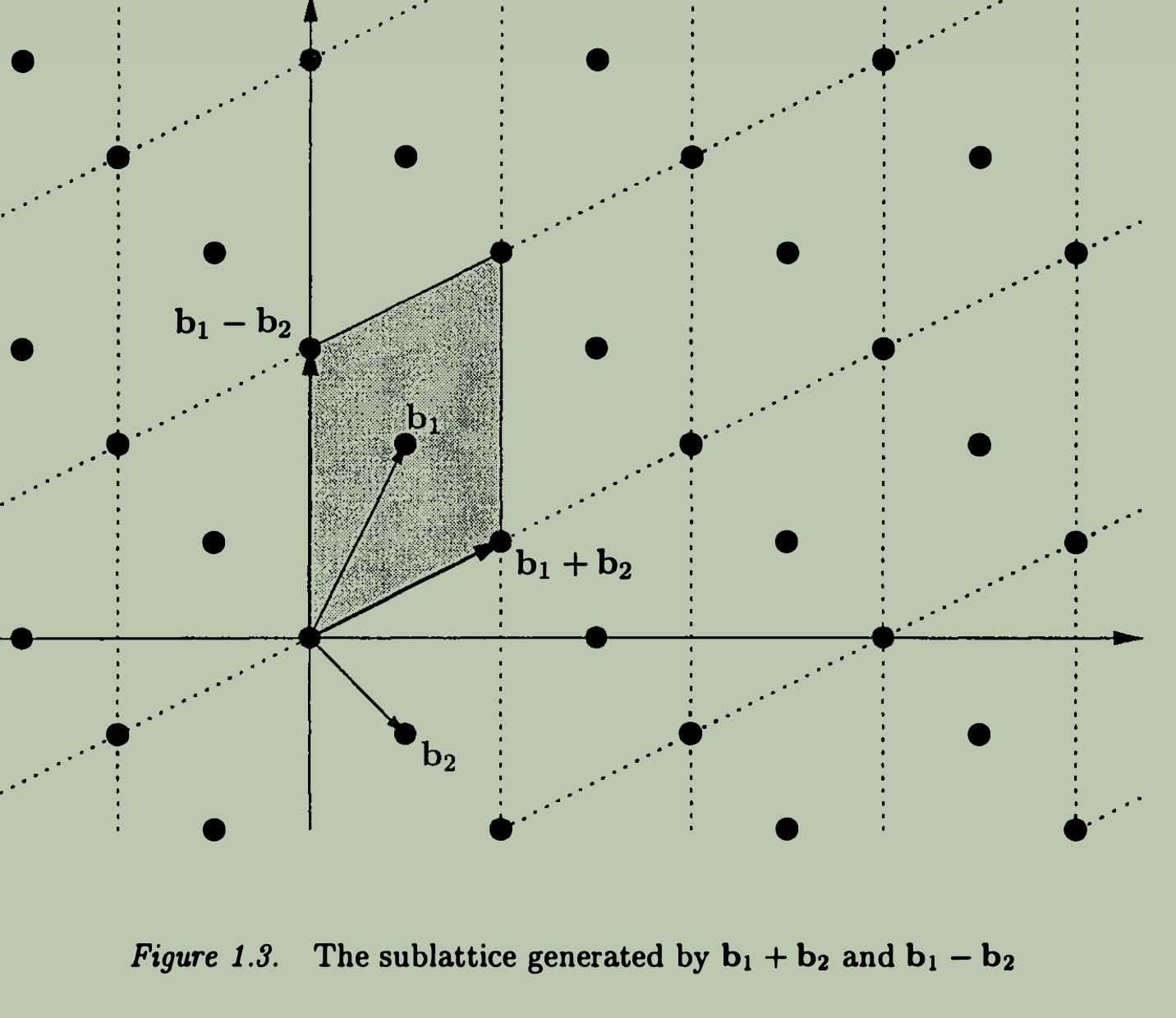
For example, two vectors from a lattice $\Lambda = \mathcal{L}(b_1, b_2)$, $$ b_1′ = b_1 + b_1 = [2, 1]^\top \\ b_2′ = b_1 – b_2 = [0, 3]^\top $$ are independent, they are surely able to form a basis for vector space $\text{span}(b_1, b_2) = \mathcal{span}(\Lambda)$. But they cannot generate the lattice $\Lambda$ since $b_1 = \frac{1}{2} (b_1′ + b_2′)$, not an integer combination of $b_1’$ and $b_2’$.
Note
So what is the characteristic of vectors that can form a lattice basis? How to remove the non-integer linear combinations from consideration?
Fact 1.2 – Valid Lattice Basis
Given a lattice $\mathcal{L}(B)$ with basis $B = [b_1, …, b_n]$, and $n$ linearly independent lattice vectors, $$ B’ = [b_1′, …, b_n’], b_i’ \in \mathcal{L}(B) $$ We define $$ \mathcal{P}(B’) = \left\{ \sum_{i=1}^n x_i b_i’ : 0 \leq x_i < 1 \right\} $$ as the half-open parallelepiped generated by the basis $B’$. Note that the coefficients $x_i$ are restricted to the interval $[0, 1)$, which ensures that each point in $\mathcal{P}(B’)$ is uniquely represented. Then $B’$ is a lattice basis if and only if $\mathcal{P}(B’)$ does not contain any lattice vector (points) other than the zero vector (origin point).
Note
If $B’$ is not a lattice basis for $\mathcal{L}(B)$, i.e., $\mathcal{L}(B’) \ne \mathcal{L}(B)$. Since it is still linearly independent, so it also generates a lattice $\mathcal{L}(B’)$ which is different from $\mathcal{L}(B)$. But, what is the relationship between $\mathcal{L}(B)$ and $\mathcal{L}(B’)$?
Fact 1.3 – Sublattice
Sublattice is an natural concept after half-open parallelepiped, if there are lattice points from $\mathcal{L}(B)$ in the half-open parallelepiped, which implies a inclusion relationship : $$ \mathcal{L}(B’) \subseteq \mathcal{L}(B). $$ If $\mathcal{L}(B’) \subsetneq \mathcal{L}(B)$, then we call $\mathcal{L}(B’)$ a proper sublattice of $\mathcal{L}(B)$.
Note
As we know the lattice basis vector is defined over $\mathbb{R}$. For the convenience of computation, we often consider lattice basis vectors over $\mathbb{Z}$, i.e., integer lattice basis vectors.
Fact 1.4 – Lattice as a Subgroup
It is obvious that a lattice $\mathcal{L}(B)$ has property of addition closure and contains the zero vector, i.e., $$ \mathbf{0} \in \mathcal{L}(B), \quad \text{and} \quad \forall u, v \in \mathcal{L}(B), \; u + v \in \mathcal{L}(B). $$ Moreover, for any $u \in \mathcal{L}(B)$, its additive inverse $-u$ is also in $\mathcal{L}(B)$. Therefore, a lattice $\mathcal{L}(B)$ forms a subgroup of the additive group $(\mathbb{R}^n, +)$.
Determinant
Definition of Determinant of a Lattice
The determinant of a lattice $\mathcal{L}(B)$, denoted as $\det(\mathcal{L}(B))$, geometrically is the volume of the fundamental parallelepiped generated by the basis $B$, i.e., $$ \det(\mathcal{L}(B)) = \text{Vol}(\mathcal{P}(B)). $$ Furthermore, the determinant of a lattice is independent of the choice of basis. That is, if $B$ and $B’$ are two different bases of the same lattice $\mathcal{L}(B)$, $\mathcal{L}(B) = \mathcal{L}(B’)$, then $$ \det(\mathcal{L}(B)) = \det(\mathcal{L}(B’)). $$ Intuitively, the determinant is the shaded area of the fundamental parallelepiped generated by the basis $B$ shown in the figures above.
A natural question is how to compute the determinant of a lattice given one basis? There are two solutions for this.
Gram-Schmidt Process
The natural way is to :
- compute the orthogonal basis $B^* = (b_1^*, …, b_n^*)$ corresponding to the given basis $B = (b_1, …, b_n)$ using the Gram-Schmidt process.
- take the product of the norms of the orthogonal basis vectors to obtain the determinant: $$ \det(\mathcal{L}(B)) = \prod_{i=1}^n \|b_i^*\|, $$ where $b_i^*$ are the Gram-Schmidt orthogonalized vectors of the basis $B$.
Take the figure 1.1 as an example, after applying the Gram-Schmidt process to the basis vectors, we obtain : $$ \begin{aligned} b_1^* &= b_1 \\ b_2^* &= b_2 – \frac{\langle b_2, b_1^* \rangle}{\langle b_1^*, b_1^* \rangle} b_1^* \\ \end{aligned} $$ where $\langle b_1^*, b_2^* \rangle = 0$. Even though the "shaded" area is a parallelogram, after being orthogonalized, it is a rectangle with area equal to the product of two orthogonal edges which corresponds to the product of the norms of the orthogonalized vectors.
Note
By Gram-Schmidt orthogonalization, we can obtain a orthogonal basis $B^*$ from any given basis $B$, if $B$ is a lattice basis, i.e., $B \in \mathcal{L}(B)$. It is obvious that some orthogonal basis vector $b_i^*$ might not be in the lattice space anymore, i.e., $b^* \notin \mathcal{L}(B)$, since the coefficients $\frac{\langle b_i, b_j^* \rangle}{\langle b_j^*, b_j^* \rangle}$ might not be an integer.
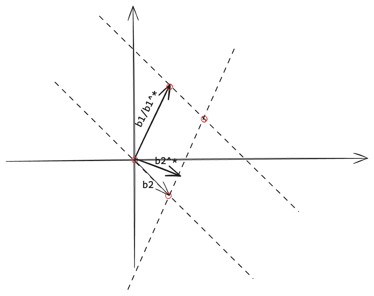
We see that $B^* = (b_1^*, b_2^*)$ is not a lattice basis since one point from $\mathcal{L}(B)$ does lie in $\mathcal{L}(B^*)$, which implies that $\mathcal{L}(B^*) \ne \mathcal{L}(B)$.
Determinant of Lattice Basis Matrix
In linear algebra, we know that, if $B = (b_1, …, b_n)$ is a basis of $\text{span}(B)$, then the determinant of the matrix formed by the basis vectors is equal to the product of the norms of the Gram-Schmidt orthogonalized vectors and a sign factor: $$ \det (B) = (-1)^{\sigma} \cdot \prod_{i=1}^n \|b_i^*\| $$ If $B$ is a lattice basis, then the determinant of the lattice $\mathcal{L}(B)$ is equal to the absolute value of the determinant of the basis matrix: $$ \det(\mathcal{L}(B)) = \prod_{i=1}^n \|b_i^*\| = |\det(B)| = \sqrt{B^T B} $$ This is an alternative way to compute the determinant of a lattice given its basis, instead of computing every orthogonal vectors sequentially.
Successive Minima
Let $\mathcal{L}(B)$ be a lattice generated by the basis $B$ with rank $n$. The $i$-th successive minimum $\lambda_i(\mathcal{L}(B))$ is defined as: $$ \lambda_i(\mathcal{L}(B)) = \inf \{ r > 0 : \dim(\text{span}(\mathcal{L}(B) \cap B(0, r))) \ge i \} $$ Intuitively, the $i$-th successive minimum represents the smallest radius of a ball centered at the origin that contains at least $i$ linearly independent lattice vectors.
More specially, when $i = 1$, the first successive minimum $\lambda_1(\mathcal{L}(B))$ corresponds to the length of the shortest non-zero lattice vector in $\mathcal{L}(B)$ : $$ \lambda_1(\mathcal{L}(B)) = \min \{\|v\| : v \in \mathcal{L}(B) \setminus \{0\}\} $$
Note
The successive minima $\lambda_i(\mathcal{L}(B))$ is independent of the choice of the lattice basis $B$, but the orthogonal basis obtained from Gram-Schmidt orthogonalization does have a relationship with the first successive minimum $\lambda_1(\mathcal{L}(B))$.
Fact 1.5 – First Successive Minimum as an Upper Norm Bound of Lattice Basis
Let $B$ a lattice basis, and let $B^*$ be the corresponding Gram-Schmidt orthogonalized basis. Then, the first successive minimum $\lambda_1(\mathcal{L}(B))$ provides an upper bound for the norms of the vectors in $B^*$: $$ \text{min}_j \|b_j^*\| \le \lambda_1(\mathcal{L}(B)), \quad \forall i = 1, …, n $$
Proof
For simplicity, we only consider a basis of a two-dimensional lattice, i.e., $B = (b_1, b_2)$. The Gram-Schmidt orthogonalized basis is $B^* = (b_1^*, b_2^*)$. By definition, we have: $$ b_1^* = b_1, \quad b_2^* = b_2 – \frac{\langle b_2, b_1^* \rangle}{\|b_1^*\|^2} b_1^* $$
Suppose any non-zero lattice vector $v = c_1 b_1 + c_2 b_2$ where $c_1, c_2 \in \mathbb{Z}$. Since $\text{span}(b_1^*, b_2^*) = \text{span}(b_1, b_2)$, any lattice vector can also be expressed as a linear combination of the Gram-Schmidt orthogonalized basis vectors: $$ \begin{aligned} v &= c_1 b_1^* + c_2 \cdot (b_2^* + \frac{\langle b_2, b_1^* \rangle}{\|b_1^*\|^2} b_1^*) \\ &= (c_1 + c_2 \frac{\langle b_2, b_1^* \rangle}{\|b_1^*\|^2}) b_1^* + c_2 b_2^* \end{aligned} $$
Two cases involved:
(a) If $c_2 \ne 0$, $v$’s component perpendicular to orthogonal basis vector $b_1^*$ is given by: $$ v_{\perp b_1^*} = c_2 b_2^* $$ thus we have $\| v \| \ge \| v_{\perp b_1^*} \| = |c_2| \|b_2^*\| \ge \|b_2^*\|$.
(b) If $c_2 = 0$, $v$ is parallel to $b_1^*$, thus we have $\| v \| \ge \| v_{\perp b_2^*} \| = |c_1| \|b_1^*\| \ge \|b_1^*\|$.
This implies for any non-zero lattice vector $v$, we have: $$ \| v \| \ge b_1^* \text{ or } \| v \| \ge b_2^* $$ which is equivalent with $$ \| v \| \ge \min_j \| b_j^* \| $$
More specially, for the first successive minimum $\lambda_1(\mathcal{L}(B))$ which is the smallest non-zero lattice vector norm, we have: $$ \lambda_1(\mathcal{L}(B)) \ge \text{min}_j \| b_j^* \| $$
Minkowski’s Theorem
Blichfeldt’s Theorem
Let $\Lambda$ be a lattice, and let $S \subset \text{span}(\Lambda)$ be a measurable set with volume $\text{vol}(S) > \det(\Lambda)$. Then, there exist two distinct points $x, y \in S$ such that $x – y \in \Lambda$.
Proof
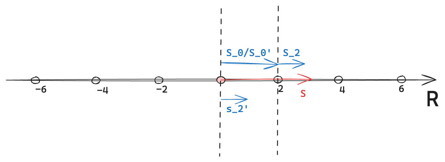
Let $\Lambda = 2 \mathbb{Z}$ be the lattice of even integers on x-axis, and $\mathcal{P}(\Lambda) = [0, 2)$ is a fundamental parallelepiped of the lattice (with only one basis vector $2$). Consider a measurable set $S = [0, 3) \subseteq \text{span}(\Lambda) = \mathbb{R}$, which ensures $\text{vol}(S) = 3 > \det(\Lambda) = 2$, then we need to show that exists $x, y \in [0, 3)$ such that $x – y \in \Lambda$.
Note that lattice $\Lambda$ is a set of discrete even points on x-axis, and $S$ is real interval on x-axis. A few facts on this :
-
The entire vector space $\mathbb{R} = \text{span}(\Lambda)$ is partitioned into disjoint translates of the fundamental parallelepiped $\mathcal{P}(\Lambda)$, i.e., $\Lambda + \mathcal{P}(\Lambda) = \mathbb{R}$ : $$ \begin{aligned} \mathbb{R} = \text{span}(\Lambda) &= \bigcup_{x \in \Lambda} (x + \mathcal{P}(\Lambda)) \\ &= [0, 2) \cup [2, 4) \cup [4, 6) \cup \dots \end{aligned} $$
-
The projections on these disjoint translates of the fundamental parallelepiped cover the entire set $S$. That is, $$ S = \bigcup_{x \in \Lambda} \big( S \cap (x + \mathcal{P}(\Lambda)) \big) $$ In our example, $S = S_0 + S_2 = [0, 2) + [2, 3)$.
-
$\text{vol}(S) > \det(\Lambda)$ ensures that there exist at least two points in $S$ that differ by a lattice vector, we can use the pigeonhole principle to guarantee this. In our example,
$$ \text{vol}(S) = \text{vol}(S_0) + \text{vol}(S_2) = 2 + 1 = 3 > \det(\Lambda) = 2 $$ Therefore, there must exist two points $x \in S_0$ and $y \in S_2$ such that $x – y \in \Lambda$. For instance, $x = 0.5 \in S_0$ and $y = 2.5 \in S_2$, then $x – y = -2 \in \Lambda$.
Convex Body Theorem
For any lattice $\Lambda$ of rank $n$ and any convex set $S \subset \text{span}(\Lambda)$ symmetric about the origin, if $\text{vol}(S) > 2^n \det(\Lambda)$, then $S$ contains a non-zero lattice point of $\Lambda$.
Proof
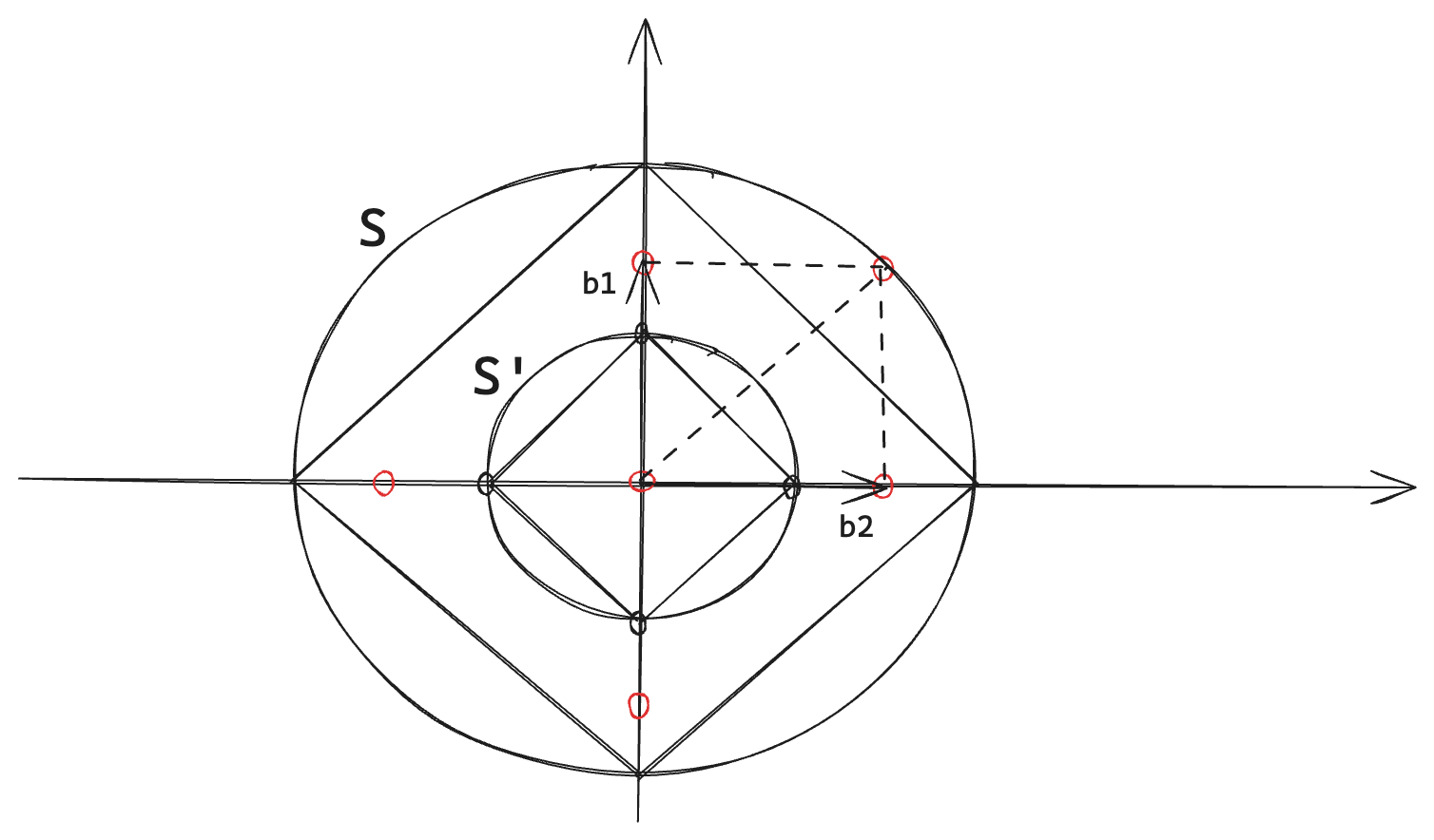
Consider another set $S’ = \{x \in \mathbb{R}^n \mid 2x \in S\}$, whose volume : $$ \text{vol}(S’) = \frac{1}{2^n} \text{vol}(S) $$ Since $\text{vol}(S) > 2^n \det(\Lambda)$, it follows that $$ \text{vol}(S’) = \frac{1}{2^n} \text{vol}(S) > \det(\Lambda) $$ By Blichfeldt’s Theorem, there exist two distinct points $x, y \in S’$ such that $x – y \in \Lambda$. Since $S’$ is a scaled version of $S$, we have $2x, 2y \in S$. Since $S$ is symmetric, then $-2x, -2y \in S$, and since $S$ is also convex, so the mid-point $\frac{2x + (-2y)}{2} = x – y \in S$. Therefore, $S$ contains a non-zero lattice point of $\Lambda$.
By observing the figure above, we can see that :
- The symmetric convex $S = \mathcal{B}(0, \sqrt{n} \det(\Lambda)^{1/n})$ be a balll of radius $\sqrt{n} \det(\Lambda)^{1/n}$ centered at the origin.
- $\text{vol}(S) > 2^n \det(\Lambda)$ always holds because it contains an $n$-dimensional hypercube with edges of length $2 \det(\Lambda)^{1/n}$. So $\text{vol}(S)$ always exceeds $(2 \det(\Lambda)^{1/n})^n = 2^n \det(\Lambda)$.
- By Minkowski’s theorem there exists a non-zero lattice point in $S$, that is $v \in \mathcal{L}(B) \setminus \{0\}$, and $\| v \| \lt \sqrt{n} \det(\Lambda)^{1/n}$. Therefore, the shortest nonzero lattice has length : $$ \lambda_1(\Lambda) \le \| v \| \lt \sqrt{n} \det(\Lambda)^{1/n} $$
By now, we have established an upper bound on the length of the shortest nonzero lattice vector in terms of the determinant of the lattice and the dimension.
Minkowski’s Second Theorem
For any rank $n$ lattice $\mathcal{L}(B)$, the successive minima (in the $l_2$ norm) $\lambda_1, …, \lambda_n$ satisfy : $$ (\prod_i^n \lambda_i)^{1/n} \lt \sqrt{n} \det(\mathcal{L}(B))^{1/n} $$
Proof Logic
The equivalence of the goal is : $$ \prod_i^n \lambda_i \lt (\sqrt{n})^n \det(\mathcal{L}(B)) $$ we will prove it by contradiction. We assume that $$ \prod_i^n \lambda_i \ge (\sqrt{n})^n \det(\mathcal{L}(B)) $$ then we need to find a contradiction after some inductions.
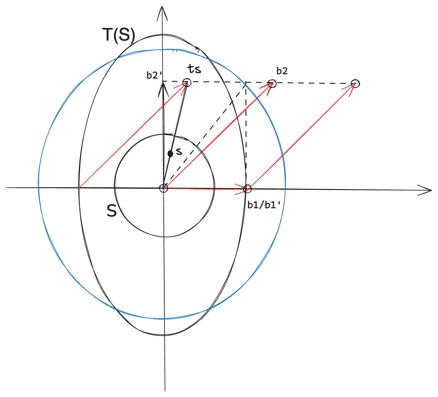
As shown in above figure, for simplicity we consider $n = 2$, a lattice $\Lambda = \mathcal{L}(B)$ with basis $B = (b_1, b_2)$ where $\| b_1 \| \le \| b_2 \|$, and successive minima $\lambda_1 = \| b_1 \|, \lambda_2 = \| b_2 \|$.
Let $S \subseteq \text{span}(\mathcal{L}(B))$ be an open (real) circle with unit radius in the real space of $\text{span}(\Lambda)$. Define a transformation that scale the horizontal axis of circle $S$ by a factor $\lambda_1$, and the vertical axis by a factor $\lambda_2$. Then we obtain an ellipse $T(S)$: $$ T((x, y)) = (\lambda_1 x, \lambda_2 y), \quad (x, y) \in S $$
If we can find a non-zero lattice point whose length is less than $\lambda_2 = \| b_2 \|$ inside the ellipse $T(S)$, then it would contradict the definition of successive minima. This is the key idea behind our proof.
It is clear that their volumn is scaled by the product of the scaling factors along each axis: $$ \text{vol}(T(S)) = \lambda_1 \cdot \lambda_2 \cdot \text{vol}(S) $$ (In 2D, the volume corresponds to the area of the ellipse, $\text{vol}(T(S)) = \pi \lambda_1 \lambda_2$ and $\text{vol}(S) = \pi$). By our assumption, $\lambda_1 \cdot \lambda_2 \ge (\sqrt{2})^2 \det(\mathcal{L}(B)) = 2 \det(\mathcal{L}(B))$, and $\text{vol}(S) = \pi > 2$, we have: $$ \text{vol}(T(S)) \gt (2 \text{vol}(S)) \cdot \det(\mathcal{L}(B)) \gt 2^2 \det(\mathcal{L}(B)) $$ Since the ellipse $T(S)$ is convex and symmetric with respect to the origin, all conditions of Minkowski’s convex body theorem are satisfied, by Minkowski’s convex body theorem, the ellipse $T(S)$ must contain a non-zero lattice point of $\mathcal{L}(B)$. For example, the point $ts \in T(S)$ is a lattice point, and it is scaled by $T$ from point $s \in S$.
Let $s = (x, y)$, then $ts = (\lambda_1 x, \lambda_2 y)$, then we have : $$ |\| ts \|^2 = \| (\lambda_1 x, \lambda_2 y) \|^2 = (\lambda_1 x)^2 + (\lambda_2 y)^2 $$ By successive minima, $\lambda_1 \le \lambda_2$ and the length of $s$ is at most 1 (since $s$ lies on the unit circle), we have : $$ \| ts \|^2 = (\lambda_1 x)^2 + (\lambda_2 y)^2 \le \lambda_2^2 (x^2 + y^2) \lt \lambda_2^2 $$ Thus $\| ts \| \lt \lambda_2$ breaks the successive minima condition, leading to a contradiction.
Computational Problems
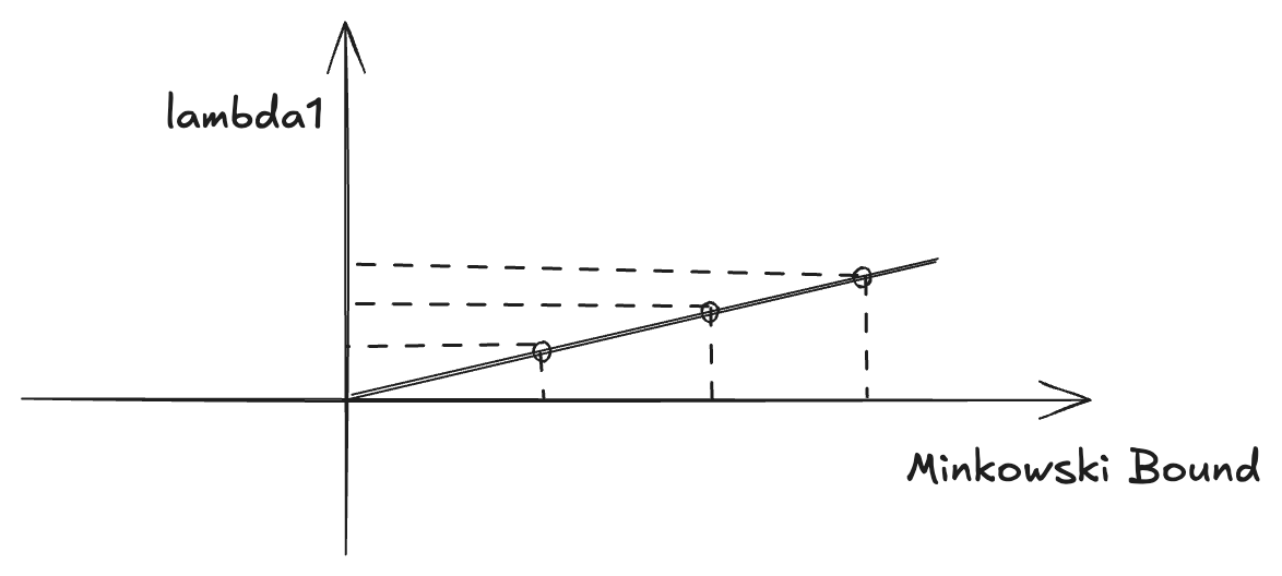
Minkowski’s bound is asymptotically tight in worst case.
That means for some lattice, the actual $\lambda_1$ is propotional to the Minkowski’s bound by some factor $0 < c < 1$: $$ \lambda_1 \approx c \cdot \sqrt{n} \det(\mathcal{L})^{1/n} $$ In this case, when $n$ grows, the Minkowski's bound also grows, and the actual $\lambda_1$ grows proportionally, but by a smaller factor $c$. But the ratio between the actual $\lambda_1$ and the Minkowski's bound remains unchanged.
Same Lattice Problems
The problem of finding a lattice vector of length $\lambda_1$ is known as the Shortest Vector Problem (SVP).
Given a lattice vector $t$, finding a nonzero lattice vector such that $\| v – t \|$ is minimized is known as the Closest Vector Problem (CVP).
Approximate SVP
Given a basis $B \in \mathbb{Z}^{m \times n}$, find a nonzero lattice vector $Bx$ where $x \in \mathbb{Z}^n \setminus \{0\}$, such that $\| Bx \| \le \gamma \cdot \| B y \|$ for any other nonzero lattice vector $By$.
Approximate CVP
Given a basis $B \in \mathbb{Z}^{m \times n}$ and a target vector $t \in \mathbb{R}^m$, find a lattice vector $Bx$ where $x \in \mathbb{Z}^n$, such that $\| Bx – t \| \le \gamma \cdot \| By – t \|$ for any other lattice vector $By$.
Solving SVP in Dimension 2
Reduced Basis
Definition 2.1 – Let $[a, b]$ be a lattice basis. The basis is reduced if
$$ |\| a \|, \| b \| \le \| a + b \|, \| a – b \| $$
Intuition Behind
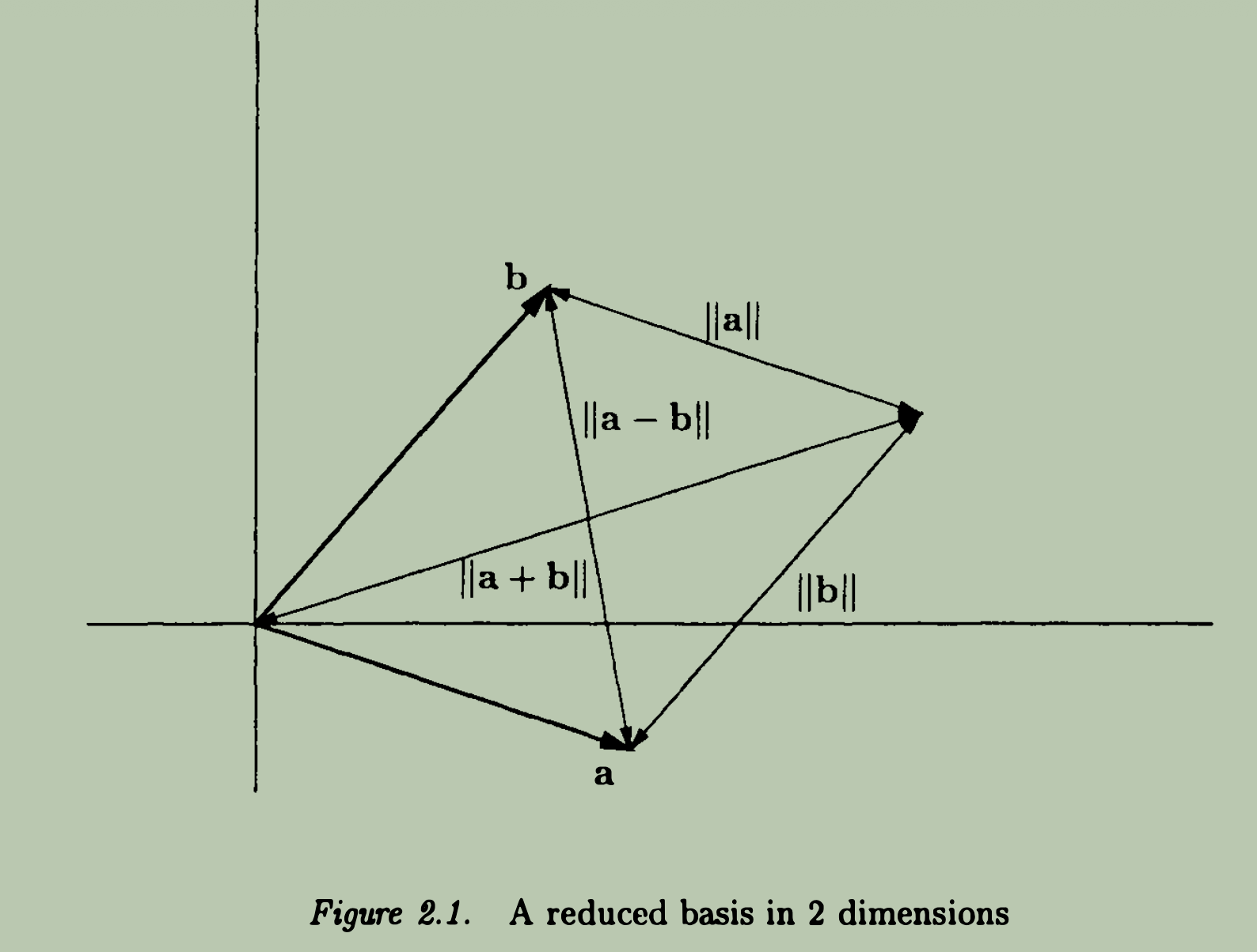
Consider constructing a triangle with known two edges $a$ and $b$, the third edge is unknown. If $[a, b]$ is reduced, by definition, we can say that $a, b$ are the shortest two edges of the triangle.
Lemma 2.1 – Consider three vectors on a line, $x, x + y, x + ay$, where $a \in \mathbb{R}$. Then if $\| x \| \le \| x + y \|$ then $\| x + y \| \le \| x + ay \|$, moreover $\| x + y \| \le \| x + ay \|$.
Explanation
Intutively, given $x, x + y$, if $\| x \| \le \| x + y \|$, then we are clear that both $x$ and $y$ are pointing in roughly the same direction, and adding any multiple of $y$ to $x + y$ will only increase the norm.
Similarly, if $\| x \| \le \| y – x \|$, then $y$ and $x$ are pointing in roughly the contradictory direction, furthermore, $\| x \| \le \| y – x \| \le \| ay – x \|$.
Important
So what is the relationship between reduced basis and the successive minima of the lattice?
Theorem 2.2 – Let $[a, b]$ be a lattice basis, and let $\lambda_1$ and $\lambda_2$ be the successive minima of the lattice. If the basis is reduced, then $\| a \| = \lambda_1$ and $\| b \| = \lambda_2$.
Explanation
From the definition of reduced basis, we know that whether $a$ and $b$ have the same direction or not, we need to ensure that either of $a$ or $b$ is the shortest vector in the lattice. Without loss of generality, we assume $\| a \| \le \| b \|$ :
- if $a, b$ have the same direction, then $\| b \| \le \| a + b \|$.
- if $a, b$ have the opposite direction, then $\| b \| \le \| a – b \|$.
put them together, we need to ensure $\| b \| \le \min \{ \| a + b \|, \| a – b \| \}$. Therefore,
$$ \| a \| \le \| b \| \le \min \{ \| a + b \|, \| a – b \| \} $$ In general, we have
$$ \| a \|, \| b \| \le \| a + b \|, \| a – b \| $$ namely, basis $[a, b]$ is reduced.
Gauss Algorithm
Definition 2.2 – For a lattice basis $[a, b]$, without loss of generality, we assume $\| a \| \le \| b \|$, if $\| a \| \le \| a – b \| \le \| b \|$, then we call the basis $[a, b]$ a well-ordered basis.
Algorithm
Explanation
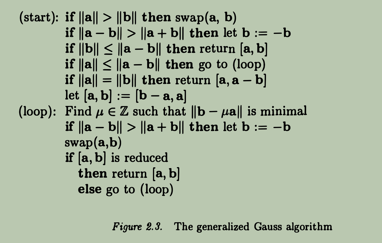
For the line-1 and line-2, we are trying to ensure
- lattice vector $a$ is the smaller one, i.e., $\| a \| \le \| b \|$
- both lattice vectors $a$ and $b$ are in the same direction, i.e., $\| a – b \| \le \| a + b \|$.
After then we will consider following cases :
-
For the line-3, it is the simplest case where $\| b \| \le \min \{ \| a + b \|, \| a – b \| \} = \| a – b \|$, in this case, we must have : $$ |\| a \| \le \| b \| \le \| a – b \| \le \| a + b \| $$ then the basis $[a, b]$ is strictly reduced, and they are in the same direction, return $[a, b]$.
-
For the rest of lines, it is the case of $\| a – b \| \lt \| b \|$, there are two subcases to consider:
-
(2.1) for the line-4, $\| a \| \le \| a – b \| \lt \| b \|$, then basis $[a, b]$ is a typical well-ordered basis, and they are in the same direction.
-
(2.2) for line-5 and line-6, $\| a – b \| \le \| a \| \le \| b \|$, then there are two subcases to consider :
-
(2.2.1) for the line-5, $\| a – b \| \le \| a \| = \| b \|$, this is a very special case, $\|a \| = \| b \|$ and $\| a – b \| \le \| a \|$ ensure that vectors $a – b$ and $a$ are in the same direction, in this case, $\| a \| = \| b \| \le \| 2a – b \|$. Since $\| (a – b) – a \| = \| b \|$, thus the basis $[a – b, a]$ is reduced, and they are in the same direction, return $[a – b, a]$.
-
(2.2.2) from line-6, $\| a – b \| \le \| a \| < \| b \|$, we do not know the whether $a - b$ and $a$ are in the same direction or not, but $\| a \| \le \| b \|$ and $\| a - b \| \le \| a \|$ ensures that vectors $b - a$ and $a$ are in the same direction, so $\| b - a \| \le \| (b - a) - a \| \le \| a \|$. Therefore, the basis $[b - a, a]$ is well-ordered basis.
-
-
The remaining problem is how to find the reduced basis through well-ordered basis in the loop :
-
Since $[a, b]$ is a well-ordered basis, there are other lattice vectors that can be fit between $[\| a \|, \| b \|]$, what we need to do is finding the smallest one. This is achieved by find the integer $\mu$ such that $\| b – \mu a \|$ is minimal, then replace $b$ with $b – \mu a$.
-
Now we can check that if the updated basis $[a, b]$ is reduced, but before checking we need to make sure that $\| a \| \le \| b \|$, if not, swap $a$ and $b$.
-
repeat the above steps until the basis $[a, b]$ is reduced.
Next, we will focus on how to find the minimal vector between two well-ordered basis vectors in the Gauss loop.
Minimal Vector in Gauss Loop
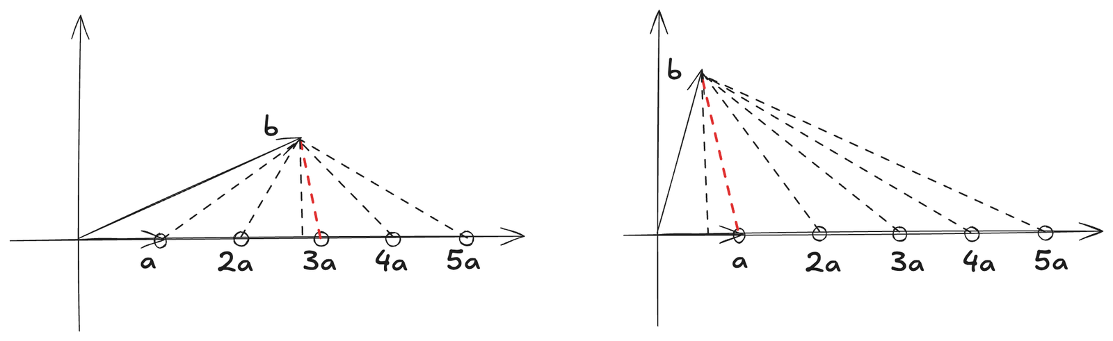
Lemma 2.3 – Let $a, b$ be two vectors such that $\| b – a \| < \| b \|$. Then, one can efficiently find an integer $\mu$ such that $\| b - \mu a \|$ is minimal. Moreover, $\mu$ satisfies $1 \le \mu \le \lceil 2\frac{\| b \|}{\| a \|} \rceil$.
Explanation
Note that, in Gauss algorithm, before entering the loop, we have ensured that the basis $[a, b]$ is well-ordered, i.e., $\| a \| \le \| b \|$ and $\| a \| \le \| a – b \| \le \| b \|$. But, this theorem does only mentioned last-half condition of well-ordered basis, i.e., $\| a – b \| \le \| b \|$. So this is a more general setting than the well-ordered basis condition.
For better understanding Gauss algorithm, we will specially consider the l2 norm, and explain why we are able to find the minimal vector between $a$ and $b$ in Gauss loop if $[a, b]$ is well-ordered with geometric intuition.
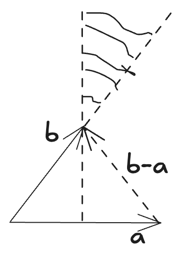
Condition $\| a \| \le \| a – b \| < \| b \|$ implies :
- vectors $a, b$ are in the same direction.
- projection scalar of $b$ onto $a$, i.e., $\frac{\langle a, b \rangle}{\| a \|^2} > 1/2$.
- the minimal distance between $b$ and $a$ is $\| b – \frac{\langle a, b \rangle}{\| a \|^2} a \|$.
Two cases involved in finding the optimal integer $\mu$ are:
- If $\frac{1}{2} < \frac{\langle a, b \rangle}{\| a \|^2} \le 1$, then $\| b - \mu a \|, u \in \mathbb{N}$ increases as $\mu$ moves away from the minimal value $\frac{\langle a, b \rangle}{\| a \|^2}$. In this case, $\mu = 1$ is the optimal integer choice.
- If $\frac{\langle a, b \rangle}{\| a \|^2} > 1$, then $\| b – \mu a \|, u \in \mathbb{N}$ increases in the range $[1, \frac{\langle a, b \rangle}{\| a \|^2})$, and decreases in the range $(\frac{\langle a, b \rangle}{\| a \|^2}, \infty)$. In this case, the optimal integer choice must come from either $\lfloor \frac{\langle a, b \rangle}{\| a \|^2} \rfloor$ or $\lceil \frac{\langle a, b \rangle}{\| a \|^2} \rceil$.
Additionally, we will simply explain why $\frac{\langle a, b \rangle}{\| a \|^2} > 1/2$ in the contex of well-ordered basis with one diagraph below.

Why Gauss Loop Works
For now, we have only illustrated how Gauss loop works, and more specially how to find the minimal vector between two well-ordered basis vectors in the Gauss loop. But we have not touched why the loop works? or why we are able to eventually reach a reduced basis through repeated iterations from a well-ordered basis.
We know that the first step of Gauss loop is to find the minimal vector between the two basis vectors $a$ and $b$ which are well-ordered, i.e., $b’ = b – \mu a$, where $\mu$ is the integer that minimizes $\| b – \mu a \|$. Theoretically, the new vector $b’$ could be :
- $\| a \| \le \| b’ \|$,
- $\| b’ \| \lt \| a \|$.
For the condition (1), since $\| b’ \| = \| b – \mu a \|$ is minimized, so :
- $\| b – \mu a \| \le \| b – (\mu – 1) a \|$ implies $\| b’ \| \le \| b’ + a \|$
- $\| b – \mu a \| \le \| b – (\mu + 1) a \|$ implies $\| b’ \| \le \| b’ – a \|$
Thus, if $\| a \| \le \| b’ \|$, then basis $[a, b’]$ is already reduced. The Gauss loop will terminate for this pair of vectors.
For the condition (2), we know that step two of Gauss loop ensures that $b’$ and $a$ are in the same direction by flipping the sign of the new vector $b’$ if necessary, i.e., $\| b’ – a \| \le \| b’ + a \|$. Since $\| b’ \| \lt \| a \|$, we have $\| b’ – a \| \le \| a \|$, furthermore, $\| b’ \| \le \| b’ – a \| \le \| a \|$. Therefore, basis $[b’, a]$ is well-ordered.
Then the Gauss loop will continue with the new well-ordered basis $[b’, a]$, repeating the process until a reduced basis is obtained.
Gauss Running Time Analysis
By analysing the Gauss loop, we know that given input well-ordered basis $[b, c]$, we can obtain a new well-ordered basis $[a, b]$ unless the basis is already reduced. Note that, in one iteration vector $b$ not changed, only vector $a$ is invented. Then repeating the process more times will eventually lead to a reduced basis. So our concern is : is the number of iterations (time complexity) bounded by a polynomial of the input size $N$ (bits of one vector entry)? The answer is yes, but before our final conclusion, a lemma is needed.
Suppose the first input basis vector is $[a_{n – 1}, a_n]$, next input is $[a_{n – 2}, a_{n – 1}]$, …, till the last input is $[a_1, a_2]$, and $[a_1, a_2]$ is reduced.
Lemma 2.4 – For $i \ge 3$, $\| a_i \| \le 1/2 \| a_{i + 1} \|$.
Explanation
Let $[a, b, c] = [a_{i – 1}, a_i, a_{i + 1}]$, given input well-ordered basis $[b, c]$ output another well-ordered basis $[a, b]$. Then we need to show the input lengths satisfy $\| b \| \le 1/2 \| c \|$.
As we know, $a = \pm(c – \mu b)$ for some integer $\mu$ that minimizes $\| a \|$. We can consider it with following cases :
- $\mu = 1$
- $\mu = 2$
- $2 \le \mu$
We omit the details proof here.
Given the input basis $[a, b]$ of Gauss algorithm, and $[a_{k}, a_{k + 1}]$ is the first well-ordered basis entering the Gauss loop, after $k$ iterations, we obtain the following inequality : $$ 2^{k – 2} \le 2^{k – 2} \| a_{3} \| \le \| a_{k + 1} \| \le \| a \| + \| b \| $$ Since before entering the Gauss loop, we may have swapping, negation, or substrating operations, but : $$ \| a_{k + 1} \| \le \| a \| + \| b \| $$ always holds. It is clear that the number of iterations is bounded : $$ k \le \log_2 (\| a \| + \| b \|) + 2 $$ If the number of bits of one vector entry is $N$, suppose there are $m$ entries in one vector, then : $$ \| a \| \le \sqrt{m \cdot (2^N \cdot 2^N)} = \sqrt{m} \cdot 2^N $$ So we have : $$ k \le (N + 3) + \log_2 \sqrt{m} $$ As $m$ is fixed, the term $\log_2 \sqrt{m}$ is constant, so $k = O(N)$.
Approximating SVP in Dimension n
Similar with the Gauss algorithm for dimension 2, the LLL basis reduction algorithm aims to find a reduced basis for higher-dimensional lattices. The definition of reduced basis in higher dimensions involves conditions on the Gram-Schmidt orthogonalization of the basis vectors and certain size-reduction criteria.
A basis $B = [b_1, …, b_n] \in \mathbb{R}^{m \times n}$ is LLL-reduced with parameter $\delta$ if it satisfies the following conditions:
- $\mu_{i, j} \le 1/2$ for all $1 \le j < i \le n$, where $\mu_{i, j}$ are the Gram-Schmidt coefficients defined by $$ \mu_{i, j} = \frac{\langle b_i, b_j^* \rangle}{\langle b_j^*, b_j^* \rangle}, $$ and $b_j^*$ are the Gram-Schmidt orthogonalized vectors of $b_j$.
- for any pair of consecutive Gram-Schmidt vectors $b_i^*$ and $b_{i-1}^*$, the Lovász condition holds: $$ \delta \| \pi_i(b_i) \|^2 \le \| \pi_i(b_{i + 1}) \|^2 $$ where $\pi_i$ denotes the projections except the first $i-1$ Gram-Schmidt vectors $b_1^*, …, b_{i-1}^*$. Suppose $1 > \delta > 1/4$.
Regarding the Lovasz condition (2), we have : $$ \pi_i(b_i) = b_i – \sum_{j=1}^{i-1} \frac{\langle b_i, b_j^* \rangle}{\langle b_j^*, b_j^* \rangle} b_j^* = b_i^* $$ and $$ \pi_i(b_{i + 1}) = b_{i + 1} – \sum_{j=1}^{i-1} \frac{\langle b_{i + 1}, b_j^* \rangle}{\langle b_j^*, b_j^* \rangle} b_j^* = b_{i + 1}^* + \mu_{i+1, i} b_i^* $$ By the Lovasz condition (2), we have an relationship between adjacent Gram-Schmidt vectors: $$ (\delta – 1/4) \| b_i^* \|^2 \le \| b_{i + 1}^* \|^2 $$ In particular, we have an relationship between Gram-Schmidt vector $b_i^*$ and the first $\delta$-LLL basis reduced vector $b_1$ : $$ \| b_i^* \| \ge \sqrt{\delta – 1/4}^{i – 1} \| b_1^* \| \ge \sqrt{\delta – 1/4}^{i – 1} \| b_1 \| $$ As the shortest lattice vector has lower bound $\lambda_1 \ge \min_{i} \| b_i^* \|$, we have $$ \lambda_1 \ge \sqrt{\delta – 1/4}^{i – 1} \| b_1 \| $$
Therefore, the first vector $b_1$ of a $\delta$-LLL reduced basis provides an approximation to the shortest lattice vector within a factor of $\sqrt{\delta – 1/4}^{-(i – 1)}$: $$ \| b_1 \| \le \sqrt{\delta – 1/4}^{-(i – 1)} \lambda_1 $$
In summary, if we find the a $\delta$-LLL reduced basis for a lattice, the first basis vector $b_1$ provides an approximation to the shortest lattice vector within a factor of $\sqrt{\delta – 1/4}^{-(i – 1)}$: $$ \| b_1 \| \le \sqrt{\delta – 1/4}^{-(i – 1)} \lambda_1 $$
The LLL basis reduction Algorithm
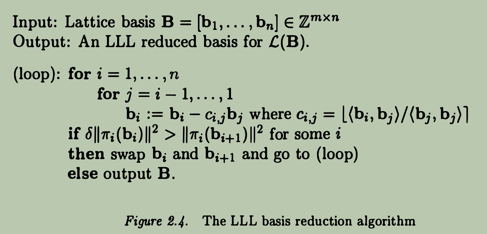
Basis Reduction
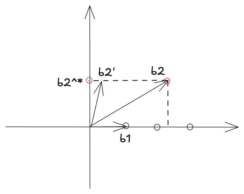
Line-1 to line-3 of LLL algorithm is to ensure that the Gram-Schmidt coefficients after reduced satisfy the size-reduction condition: $$ \mu_{i, j} \le 1/2 \quad \text{for all } 1 \le j < i \le n $$ A few facts to be noted about the size-reduction condition are:
-
To ensure that the updated basis vector $b_i$ after reduced is still a valid latice vector. We need to substract integer multiples $c_{i, j}$ of previous basis vectors $b_j$ for $j < i$, not arbitrary real multiples $\mu_{i, j}$ of orthogonal vectors $b_j^*$. In this case, the projections of $b_i$ on previous orthogonal basis vectors are not entirely eliminated, but only fraction of less than $1/2$ remains. That is, after reduced on $b_i$, it satisfies : $$ b_i = b_i^* + \sum_{j=1}^{i-1} u_{i, j} b_j^* $$ where $u_{i, j} \le 1/2$.
Notice that, there is a obvious typing error in the LLL algorithm above, that is : $$ c_{i, j} = \lfloor \mu_{i, j} \rceil = \lfloor \frac{\langle b_i, b_j^* \rangle}{\langle b_j^*, b_j^* \rangle} \rceil $$
-
Geometrically, the size-reduction condition ensures the angle between the updated basis vector $b_i$ and the actual orthogonal basis vector $b_i^*$ not too large, keeping $b_i$ relatively close to $b_i^*$ in direction.
-
The Gram-Schmidt basis vectors $b_i^*$ are not affected by the reduction process.
Lovasz Condition Check
Line-4 to line-5 of the LLL algorithm is to check the Lovasz condition, that is any consecutive Gram-Schmidt vectors satisfy $$ (\delta – 1/4) \| b_i^* \|^2 \le \| b_{i + 1}^* \|^2 $$ which ensures that the first reduced basis vector $b_1$ is not too far from the shortest lattice vector $\lambda_1$ : $$ \| b_1 \| \le \sqrt{\delta – 1/4}^{-(i – 1)} \lambda_1 $$
LLL Running Time Analysis
The running time cost is composed by two factors :
-
the number of iterations required for the algorithm to converge.
-
the computational cost of each iteration, which involves size-reduction and Lovasz condition checks for the basis vectors.
- in the reduction step, we need to round the Gram-Schmidt coefficients $$ c_{i, j} = \lfloor \mu_{i, j} \rceil = \lfloor \frac{\langle b_i, b_j^* \rangle}{\| b_j^* \|^2} \rceil $$ , which divisions of numerator and denominator of $\mu_{i, j}$ is involved. And only $b_i$ is integer valued, while the Gram-Schmidt vectors $b_j^*$ are generally not integer valued. So we need to figure the bits required for the denominator of $\mu_{i, j}$ after simplification, which not necessarily must be $\| b_j \|^2$.
- in the reduction step, we also need to update basis vector $$ b_i \leftarrow b_i – c_{i, j} b_j $$ coordinate-wise, if the rounded integer coefficient $c_{i, j}$ is too large, then the bit length of intermediate value $c_{i, j} b_j$ coordinates could become very large, affecting the overall computational cost of the reduction step even though original bit length of $b_i$ coordinates is $N$.
Bound the Number of Iterations
As we know, for any $i$, the lattice not changed through basis reduction from $B_i = [b_1, …, b_i]$ to $B’ = [b_1′, …, b_i’]$, that is : $$ \Lambda(B_i) = \Lambda(B_i’) $$ So the determinant of the lattice remains unchanged, we denote it as $\det(\Lambda_i)$. But the swap operation when the Lovasz condition is violated may change the individual Gram-Schmidt vectors, it has some effect on some sub-lattice, but the overall determinant remains the same.
For example, we suppose the reduced basis is $B = [b_1, b_2, b_3, b_4]$, if the Lovasz condition is violated for $b_2$ and $b_3$, that is : $$ \| b_3^* \|^2 < (\delta - 1/4) \| b_2^* \|^2 $$ , in this case, we have to swap $b_2$ and $b_3$. After the swap, the new basis is $B' = [b_1, b_3, b_2, b_4]$. We see that :
- lattice $\Lambda_1$ not changed, because it only involves $b_1$.
- lattice $\Lambda_2$ changed from $\mathcal{L}([b_1, b_2])$ to $\mathcal{L}([b_1, b_3])$ after the swap.
- lattice $\Lambda_3$ not change, because $\Lambda([b_1, b_2, b_3]) = \Lambda([b_1, b_3, b_2])$ even after the swap. And it does not affect the overall determinant of the lattice $\Lambda_4$.
So we define
$$
D_{i} = \det (\Lambda_i)^2 = \det([b_1, …, b_{i – 1}, b_i]) = \prod_{k=1}^{i} \| b_k^* \|^2
$$
as the squared determinant of the sub-lattice $\Lambda_i$ before swapping operation. And
$$
D_{i}^{(1)} = \det (\Lambda_i’)^2 = \det([b_1, …, b_{i – 1}, b_{i + 1}]) = \prod_{k=1}^{i – 1} \| b_k^* \|^2 \cdot (\mu_{i + 1, i} \| b_i^* \| + b_{i + 1}^*)^2
$$
as the squared determinant of the sub-lattice $\Lambda_i$ after swapping operation. Put them together, we have :
$$
\frac{D_{i}^{(1)}}{D_i} = \frac{\prod_{k=1}^{i – 1} \| b_k^* \|^2 \cdot (\mu_{i + 1, i} \| b_i^* \| + b_{i + 1}^*)^2}{\prod_{k=1}^{i} \| b_k^* \|^2} = \frac{(\mu_{i + 1, i} \| b_i^* \| + b_{i + 1}^*)^2}{\| b_i^* \|^2} \lt \delta
$$
which means the square determinant of sublattice $D_i$ decreases by a factor of at most $\delta$. But swap operation may happen position within $n$, so we need to track all possible these changes induced by swap operations. We define :
$$
\Phi_0 = \prod_{i=1}^{n} D_i
$$
as the product of the squared determinants of all sub-lattices before any swapping operation. It will drop by at most a factor of $\delta$ for any swap operation at any position $i$ within the basis :
$$
\Phi_0 \rightarrow_{i_1} \Phi_1 \rightarrow_{i_2} \Phi_2 … \rightarrow_{i_k} \Phi_k
$$
So after $k$ iterations, we have :
$$
\Phi_k \lt \delta^k \Phi_0
$$
particularly we get the relationship between iteration number $k$ and the initial product of the squared determinants of all sub-lattices $\Phi_0$ :
$$
k \lt \frac{\ln \Phi_0}{\ln (1/\delta)}
$$
For one input vector $b_i$, we have : $$ \| b_i \|^2 \le m \cdot 2^{2N} $$ , and $\| b_i^* \|^2 \le \| b_i \|^2 \le m \cdot 2^{2N}$. We can bound $\Phi_0$ in terms of input size $N$ : $$ \Phi_0 = \prod_{i=1}^{n} D_i = \prod_{i=1}^{n} \prod_{k=1}^{i} \| b_k^* \|^2 \le \prod_{i=1}^{n} (m \cdot 2^{2N})^i = (m \cdot 2^{2N})^{\frac{n(n+1)}{2}} $$ So we have : $$ \ln \Phi_0 \le \ln \left( (m \cdot 2^{2N})^{\frac{n(n+1)}{2}} \right) = \frac{n(n+1)}{2} \cdot (\ln m + 2N) $$ which is polynomial in the input size $N$ and the dimension $n$ as we expected.
Since $\delta < 1$ is a fixed number, we can just treat $\ln (1/\delta)$ as a constant. Therefore, the number of iterations $k$ is polynomially bounded in terms of the input size $N$ and the dimension $n$.
Bound the Time Cost Per Iteration
As we mentioned before, we need to bound two things :
- the bit-length of the denominator of Gram-Schmidt coefficients $\mu_{i,j}$.
- the bit-length of intermediate values after some reduction step induced by multiplying (integer) rounded Gram-Schmidt coefficients $c_{i, j}$.
Regarding (1), as we know $D_i = \prod_{k=1}^{i} \| b_k^* \|^2$, thus $\| b_j^* \|^2 = \frac{D_{j}}{D_{j – 1}}$, therefore
$$
\mu_{i, j} = \frac{\langle b_i, b_j^* \rangle}{\| b_j^* \|^2} = \frac{\langle b_i, D_{j – 1} \cdot b_j^* \rangle}{D_j}
$$
We see that vector $b_j$ coordinates are integers, and will show that :
(1.1) $D_j$ is an integer
(1.2) $D_{j – 1} \cdot b_j^*$ is integer vector
In this case, $D_j$ is divisible by the actual denominator of $\mu_{i, j}$, that is, $$ \text{denom}(\mu_{i, j}) \mid D_j $$ or $$ \text{denom}(\mu_{i, j}) \le D_j \le \Phi_0 $$ Thus the bit-length of the actual denominator of $\mu_{i, j}$ is at most the bit-length of $\Phi_0$, which is polynomially bounded in terms of the input size $N$ and the dimension $n$. That is, $$ \log \text{denom}(\mu_{i, j}) \le \log \Phi_0 \le \frac{n(n+1)}{2} \cdot (\ln m + 2N) $$
Proof of (1.1) and (1.2)
For (1.1) we can express $D_j$ with Gram matrix $B_j^T B_j$ where $B_j = [b_1, …, b_j]$, that is : $$ D_j = \det (\mathcal{L}([b_1, …, b_j])) = \det (B_j^T B_j) $$
Proof
Define $$ C_j = [b_1^*, b_2^*, …, b_j^*] $$ as the matrix whose columns are the Gram-Schmidt vectors $b_1^*, …, b_j^*$.
The relationship between Gram-Schmidt vectors $b_i^*$ and the original basis vectors $b_i$ is given by: $$ \begin{aligned} b_1 &= b_1^* \\ b_2 &= b_2^* + \mu_{2,1} b_1^* \\ b_3 &= b_3^* + \mu_{3,2} b_2^* + \mu_{3,1} b_1^* \\ \vdots \\ b_j &= b_j^* + \sum_{k=1}^{j-1} \mu_{j,k} b_k^* \end{aligned} $$ Let $$ U = \begin{matrix} 1 & \mu_{2,1} & \mu_{3, 1} & \cdots & \mu_{j,1} \\ 0 & 1 & \mu_{3,2} & \cdots & \mu_{j,2} \\ \vdots & \vdots & \vdots & \ddots & \vdots \\ \vdots & \vdots & \vdots & \ddots & \mu_{j,j-1} \\ 0 & 0 & 0 & \cdots & 1 \end{matrix} $$ be the upper triangular matrix relating the original basis vectors $b_i$ to the Gram-Schmidt vectors $b_i^*$, so we have : $$ B_j = C_j \cdot U $$ Furthermore : $$ B_j^T B_j = (C_j \cdot U)^T (C_j \cdot U) = U^T C_j^T C_j U $$ Since the columns of $C_j$ are orthogonal, thus $C_j^T C_j$ is a diagonal matrix with entries $\| b_1^* \|^2, \| b_2^* \|^2, …, \| b_j^* \|^2$ on the diagonal, that is : $$ C_j^T C_j = \text{diag}(\| b_1^* \|^2, \| b_2^* \|^2, …, \| b_j^* \|^2) $$
By the property of determinants, we have: $$ \det(B_j^T B_j) = \det(U^T C_j^T C_j U) = \det(U^T) \det(C_j^T C_j) \det(U) = (\det(U))^2 \det(C_j^T C_j) $$ Since $U$ is an upper triangular matrix with all diagonal entries equal to 1, we have $\det(U) = 1$. Therefore: $$ D_j = \det(B_j^T B_j) = \det(C_j^T C_j) = \prod_{k=1}^{j} \| b_k^* \|^2 $$
Therefore $D_j$ is an integer since it is the determinant of an integer matrix $C_j^T C_j$.
For (1.2), by Gram-Schmidt process, we have : $$ b_j^* = b_j – \sum_{k=1}^{j-1} \mu_{j,k} b_k^* $$ Unfortunately, we cannot determine if $D_{j – 1} b_j^*= D_{j – 1} b_j – \sum_{k=1}^{j-1} \langle b_j, b_k^* \rangle b_k^*$ is an integer directly since Gram-Schmidt vectors $b_j^*$ are generally not integer vectors.
We express $D_{j – 1}$ with Gram matrix $G_{j – 1} = B_{j-1}^T B_{j-1}$ where $B_{j-1} = [b_1, …, b_{j-1}]$: $$ D_{j – 1} = \det (\mathcal{L}([b_1, …, b_{j-1}])) = \det (G_{j – 1}) $$ We will show that :
a. $G_{j – 1}^{-1} = \text{adj}(G_{j – 1}) / \det(G_{j – 1}) = \text{adj}(G_{j – 1}) / D_{j – 1}$
This formula demonstrate the relationship between the inverse of the Gram matrix $G_{j – 1}$ and its adjugate and determinant, which will be useful in expressing $b_j^*$ in terms of integer matrices.
Proof of (a)
We need to show : $$ G_{j – 1} \cdot \text{adj}(G_{j – 1}) = D_{j – 1} = \det(G_{j – 1}) I $$
By Cramer’s rule, the determinant of square matrix $G_{j – 1}$ can be expressed as a linear combination of the entries of any row (or column) and their corresponding determinants of the submatrices obtained by removing the row and column of each entry : $$ \det(G_{j – 1}) = \sum_{t = 1}^{j-1} G_{{j – 1}, (r, t)} \cdot \boxed{(-1)^{r + t} \det(G_{j – 1} \setminus {[r,t]})} $$
Firstly, we define the cofactor matrix of $G_{j – 1}$ as $\text{Cof}(G_{j – 1})$, where the $(i, j)$-th entry of it is : $$ \text{Cof}(G_{j – 1})_{i,j} = (-1)^{i+j} \det(G_{j – 1} \setminus {[i,j]}) $$ where $G_{j – 1} \setminus {[i,j]}$ is the matrix obtained from $G_{j – 1}$ by removing the $i$-th row and $j$-th column. And the adjugate of $G_{j – 1}$ is defined as the transpose of the cofactor matrix: $$ \text{adj}(G_{j – 1}) = \text{Cof}(G_{j – 1})^T $$
Secondly, the $(r, s)$-th entry of the matrix $H = G_{j – 1} \cdot \text{adj}(G_{j – 1})$ is : $$ H_{r, s} = \langle G_{j – 1, (r, :)}, \text{adj}(G_{j – 1})_{(:, s)} \rangle = \langle G_{j – 1, (r, :)}, \text{Cof}(G_{j – 1})_{(s, :)} \rangle = \sum_{t = 1}^{j-1} G_{j – 1, (r, t)} \cdot (-1)^{s + t} \det(G_{j – 1} \setminus {[s, t]}) $$ Two cases arise:
- If $r = s$, then above formula is aligned with that of determinant of $G_{j – 1}$, giving $H_{r, s} = \det(G_{j – 1}) = D_{j – 1}$.
- if $r \ne s$, then $H_{r, s}$ equals the derminant of another matrix $G_{j – 1}’$ obtained by replacing the $s$-th row of $G_{j – 1}$ with a copy of the $r$-th row. Since $G_{j – 1}’$ has two identical rows, its determinant must be zero. Therefore, $H_{r, s} = 0$ for $s \ne r$. Hence, $H$ is a diagonal matrix with $D_{j – 1} = \det(G_{j – 1})$ on the diagonal.
This completes the proof of (a).
b. $b_j^* = b_j – B_{j – 1}^T G_{j – 1}^{-1} B_{j – 1} b_j$ is another expression for the Gram-Schmidt vector $b_j^*$.
Proof of (b)
In this case, we can express $D_{j – 1} b_j^*$ as: $$ D_{j – 1} b_j^* = D_{j – 1} \left( b_j – B_{j – 1}^T G_{j – 1}^{-1} B_{j – 1} b_j \right) = D_{j – 1} b_j – B_{j – 1}^T \text{adj}(G_{j – 1}) B_{j – 1} b_j $$ Since $D_{j – 1} = \det(G_{j – 1})$ and $\text{adj}(G_{j – 1})$ are integer matrices, the right-hand side is an integer vector. Therefore, $D_{j – 1} b_j^*$ is an integer vector.
Regarding (2), assume $b_i$ is the reduced basis vector, each entry is bounded by :
$$
\| b_{i, j} \|^2 \le \| b_i \|^2
$$
By Gram-Schmidt process, we can consider to bound $\| b_i \|^2$ :
$$
\| b_i \|^2 = (\| b_i^* \| + \sum_{k = 1}^{i-1} \mu_{i, k} \| b_k^* \|)^2 = \| b_i^* \|^2 + \sum_{k = 1}^{i – 1} \mu_{i, k}^2 \| b_k^* \|^2
$$
By previous definition, we have :
$$
\|b_i^*\|^2 = \frac{D_i}{D_{i-1}}
$$
since $1 \le D_i \le \Phi_0$, we have :
$$
1 / \Phi_0 \le \| b_i^* \|^2 \le \Phi_0
$$
As after reduced, the Gram-Schmidt coefficients $\mu_{i, k}$ satisfy $|\mu_{i, k}| \le 1/2$, we have:
$$
\begin{aligned}
\| b_i \|^2 &\le (1 + \sum_{k = 1}^{i – 1} (1/2)^2) \| b_i^* \|^2 \\
&= (1 + \frac{i – 1}{4}) \| b_i^* \|^2 \\
&\le (1 + \frac{i – 1}{4}) \Phi_0 \\
\end{aligned}
$$
Therefore the bit-length of each entry of $b_i$ is bounded by $O(\log \Phi_0)$ where $\log \Phi_0$ is polynomial in the input size $N$ as :
$$
\log \Phi_0 \le \frac{n(n + 1)}{2} (\log m + 2N)
$$

Pingback: Index | paynejoe.com